The Story Behind censo2017, the First rOpenSci Package to be Reviewed in Spanish

🔗Summary

censo2017 is an R package designed toorganize the Redatam¹ filesprovided by the Chilean National Bureau of Statistics (Instituto Nacional deEstadísticas de Chile in spanish) in DVD format². This package was inspiredby citesdb(Noam Ross, 2020) and taxadb(Carl Boettiger et al, 2021).This post is about thispackage, the problem it solves, how to use it, and the fact that the package andits review process were all inSpanish.

🔗The census challenge

The motivationto have completed this is that, almost two years ago now, I had to complete anassignment that required me to extract data from the aforementioned DVD and itgot very complicated.

I had to borrow a Windows laptop and get an external DVD reader in order to readthose REDATAM files to obtain a few population summaries with specific softwarefor that format. To my surprise, the task started to get more and morechallenging, to the point that I wanted to export the data to SQL for easierdata extraction.

My goal wasn't to extract statistical secrets, which is not possible with thesedatasets, I just wanted to obtain values of population by age intervals fordifferent regions, among other similar aggregations, which is something thatdplyr and other tools ease a lot. After being able to convert the datasets andthe description of variables to CSV/XML, I found that the effort in doing thatjustified creating an R package to organize my work.

🔗The long way to simplicity

The REDATAM Converter(Pablo De Grande, 2016) allows exporting complete REDATAM databases as CSV foruse in, for example, R or Python. Unfortunately, this tool is also Windows-only,and as a Linux user I wanted to make the census datasets easily available forall platforms.

Besides REDATAM, using CSV for a census is not the best choice, as that involvesreading 4 GB tables from disk. This is so big that most laptops won't be able toperform joins, no matter what tool you use (R, Python or sub-tools such as readror data.table, just to mention a few excellent tools). However, using a SQLbased tool, such as DuckDB, allows efficient querying and makes most censusoperations possible on a common laptop.

censo2017 creates a local and embedded DuckDB databasethat simplifies analysis of the census datasets. It allows efficient queryingand is accessible via a DBI compatible interface. Thepackage also provides an interactive pane for RStudiothat allows exploring the database and previewing data. The ultimate goal ofthis work is to ease data access for researchers in Humanities and SocialSciences.

🔗How does censo2017 work?

For a quick illustration, assume we haven't already installed the package andthe local database, which are two separate steps.

# install, load the package and create the local databaseremotes::install_github("ropensci/censo2017")library(censo2017)censo_descargar()# to be able to use collect() and use regular expressionslibrary(dplyr)

We know there are roughly 17 million inhabitants in Chile, but how many of themare men/women? How old are Chileans? How many of them attendeduniversity/community college? How many of them work on each branch of economicactivity³? Census questions "p08", "p09", "p15" and "p18" tell us thisinformation.

This package features a metadata table (variables) which is not a part of theoriginal files, as it was inferred from the REDATAM structure, that tells us towhich table each variable belongs. For example, by using dplyr we can look fordescriptions that match "Curso" (Course).

tbl(censo_conectar(), "variables") %>%  collect() %>%  filter(grepl("Curso", descripcion))  tabla    variable descripcion                       tipo    rango  <chr>    <chr>    <chr>                             <chr>   <chr>1 personas p14      Curso o Año Más Alto Aprobado     integer 0 - 82 personas p15      Nivel del Curso Más Alto Aprobado integer 1 - 14

Those who are familiar with these codes might remember each value for "p15", butfortunately for the rest of us, this package also attaches the labels, so anyuser can see that "p15 = 12" means "the person attended university".

tbl(censo_conectar(), "variables_codificacion") %>%  collect() %>%  filter(variable == "p15")   tabla    variable valor descripcion                                                  <chr>    <chr>    <int> <chr>                                                      1 personas p15          1 Sala Cuna o Jardín Infantil                                2 personas p15          2 Prekínder                                                  3 personas p15          3 Kínder                                                     4 personas p15          4 Especial o Diferencial                                     5 personas p15          5 Educación Básica                                           6 personas p15          6 Primaria o Preparatoria (Sistema Antiguo)                  7 personas p15          7 Científico-Humanista                                       8 personas p15          8 Técnica Profesional                                        9 personas p15          9 Humanidades (Sistema Antiguo)                             10 personas p15         10 Técnica Comercial, Industrial/Normalista (Sistema Antiguo)11 personas p15         11 Técnico Superior (1-3 Años)                               12 personas p15         12 Profesional (4 o Más Años)                                13 personas p15         13 Magíster                                                  14 personas p15         14 Doctorado                                                 15 personas p15         99 Valor Perdido                                             16 personas p15         98 No Aplica

To get detailed information for each commune/region regarding the questionsabove, we need to think of the REDATAM data as a tree, and it is necessary tojoin "zonas" (zones) with "viviendas" (dwellings) by zone ID, then join"viviendas" with "hogares" (households) by dwelling ID, and then "hogares" with"personas" (people) by household ID. This is done in no time with the DuckDBbackend.

personas <- tbl(censo_conectar(), "zonas") %>%  mutate(    region = substr(as.character(geocodigo), 1, 2),    comuna = substr(as.character(geocodigo), 1, 5)  ) %>%  select(region, comuna, geocodigo, zonaloc_ref_id) %>%  inner_join(select(tbl(censo_conectar(), "viviendas"),    zonaloc_ref_id, vivienda_ref_id), by = "zonaloc_ref_id") %>%  inner_join(select(tbl(censo_conectar(), "hogares"), vivienda_ref_id,    hogar_ref_id), by = "vivienda_ref_id") %>%  inner_join(select(tbl(censo_conectar(), "personas"), hogar_ref_id,    p08, p15, p18), by = "hogar_ref_id") %>%  collect()

A quick verification can be obtained with a count. The resulting tablemakes perfect sense and it reflects common knowledge summary statistics, such asthat in the capitol (region #13) there are around 7 million inhabitants.

personas %>%  group_by(region) %>%  count()   region       n   <chr>    <int> 1 01      330558 2 02      607534 3 03      286168 4 04      757586 5 05     1815902 6 06      914555 7 07     1044950 8 08     2037414 9 09      95722410 10      82870811 11      10315812 12      16653313 13     711280814 14      38483715 15      226068

To get to know the share of men (1) and women (2) per region,the code is very similar.

personas %>%  group_by(region, p08) %>%  count() %>%  group_by(region) %>%  mutate(p = n / sum(n))  region   p08      n     p   <chr>  <int>  <int> <dbl> 1 01         1 167793 0.508 2 01         2 162765 0.492 3 02         1 315014 0.519 4 02         2 292520 0.481 5 03         1 144420 0.505 6 03         2 141748 0.495 7 04         1 368774 0.487 8 04         2 388812 0.513 9 05         1 880215 0.48510 05         2 935687 0.515# … with 20 more rows  

At this point we obtained simple aggregations, but being R a language forstatistics, you might be interested in doing inference. As an example, assumethat the population follows a normal distribution, so that it makes sense tofind the 95% confidence interval estimate of the difference between the maleproportion of elderly people⁴ and the female proportion of non-elderlypeople, each within their own age group.

sex_vs_elder <- tbl(censo_conectar(), "personas") %>%  select(sex = p08, p09) %>%  mutate(elderly = ifelse(p09 >= 64, 1, 0)) %>%  group_by(sex, elderly) %>%  count() %>%  # labels re-arrangement, put here for efficiency  mutate(    elderly = ifelse(elderly == 1, "1. elderly", "2. non-elderly"),    sex = ifelse(sex == 1, "1. men", "2. women")  ) %>%  ungroup() %>%  collect()sex_vs_elder  sex      elderly              n  <chr>    <chr>            <dbl>1 1. men   2. non-elderly 76667282 2. women 2. non-elderly 77516763 1. men   1. elderly      9352614 2. women 1. elderly     1220338

Before conducting a proportions test, we need to re-shape the data and thenproceed with the test.

xtabs(n ~ elderly + sex, sex_vs_elder)                 sexelderly           1. men 2. women  1. elderly      935261  1220338  2. non-elderly 7666728  7751676prop.test(xtabs(n ~ elderly + sex, sex_vs_elder))  2-sample test for equality of proportions with continuity correctiondata:  xtabs(n ~ elderly + sex, sex_vs_elder)X-squared = 30392, df = 1, p-value < 2.2e-16alternative hypothesis: two.sided95 percent confidence interval: -0.06407740 -0.06266263sample estimates:   prop 1    prop 20.4338752 0.4972452

The 95% confidence interval estimate of the difference between the proportion ofmale elders and non-elders is between -6.4% and -6.3%, which is in line with thefact that women tend to have a longer life expectancy in Chile (seeStatistato compare). What I wanted to demonstrate here is that by using this package, itis very easy to pass data to R, so that you can conduct regression analysis orother statistical analyses on the Chilean population.

🔗Using censo2017 with other packages

Censo2017 can be used with ggplot2 and other commonly used packages. As an example,it is possible to replicate different overcrowding maps created by bothChile's Geographers (Geógrafas Chile) andCenter For Spatial Research (Centro de Producción del Espacio)that account for overcrowding in the Metropolitan Region.

To obtain this, you need both the number of indiduals and rooms per dwellings.You can obtain the corresponding columns in the same way as the previousexamples.

tbl(censo_conectar(), "variables") %>%  collect() %>%  filter(grepl("Pers", descripcion))  tabla     variable descripcion          tipo    rango     <chr>     <chr>    <chr>                <chr>   <chr>   1 personas  personan Número de la Persona integer 0 - 99992 viviendas cant_per Cantidad de Personas integer 0 - 9999  

You need "cantidad de personas" (number of individuals) from the "viviendas"table.

tbl(censo_conectar(), "variables") %>%  collect() %>%  filter(grepl("Dorm", descripcion))  tabla     variable descripcion                                            tipo    rango  <chr>     <chr>    <chr>                                                  <chr>   <chr>1 viviendas p04      Número de Piezas Usadas Exclusivamente Como Dormitorio integer 0 - 6

From the variables "cant_per" and "p04" you can use the methodology used bytheSecretary for Social Development and Family (Ministerio de Desarrollo Social y Familia),which consists in taking the ratio of people residing in the dwelling and thenumber of bedrooms in the dwelling. The variable is then discretized asfollows:

• No overcrowding [0,2.5)
• Mean [2.5,3.5)
• High [3.5,4.9)
• Critical [5,Inf)

You can obtain the table with the overcrowding index for each dwelling as follows.

overcrowding <- tbl(censo_conectar(), "zonas") %>%   mutate(    region = substr(as.character(geocodigo), 1, 2),    provincia = substr(as.character(geocodigo), 1, 3),    comuna = substr(as.character(geocodigo), 1, 5)  ) %>%   filter(region == 13) %>%   select(comuna, geocodigo, zonaloc_ref_id) %>%  inner_join(select(tbl(censo_conectar(), "viviendas"), zonaloc_ref_id,                     vivienda_ref_id, cant_per, p04),             by = "zonaloc_ref_id") %>%  mutate(    cant_per = as.numeric(cant_per),     p04 = as.numeric(p04),    p04 = case_when(      p04 == 98 ~ NA_real_,      p04 == 99 ~ NA_real_,      TRUE ~ as.numeric(p04)    )  ) %>%   filter(!is.na(p04)) %>%   mutate(    # Overcrowding index (variables at dwelling level)    ind_hacinam = case_when(      # this divides people by bedrooms (if bedrooms >= 1) and       # also for 0 bedrooms (where applies bedrooms + 1 for cases such as      # studio apartment, etc)      p04 >=1 ~ cant_per / p04,      p04 ==0 ~ cant_per / (p04 + 1)    )  ) %>%   mutate(    # Hacinamiento categorias    hacinam = case_when(      ind_hacinam  < 2.5                     ~ "No Overcrowding",      ind_hacinam >= 2.5 & ind_hacinam < 3.5 ~ "Mean",      ind_hacinam >= 3.5 & ind_hacinam < 5   ~ "High",      ind_hacinam >= 5                       ~ "Critical"    )  ) %>%   collect()

To obtain the shares, you can aggregate to obtain the correspondingcounts, taking into account that you don't have to ignore the zeroes, andspecially if you want to visualize the information or you'll end up withempty areas in your map. To perform this step, you can use tidyr and janitorto obtain one column per overcrowding category.

library(tidyr)library(janitor)overcrowding1 <- overcrowding %>%   group_by(geocodigo, hacinam) %>%   count()overcrowding2 <- expand_grid(  geocodigo = unique(overcrowding$geocodigo),  hacinam = c("No Overcrowding", "Mean", "High", "Critical"))overcrowding2 <- overcrowding2 %>%   left_join(overcrowding1) %>%   pivot_wider(names_from = "hacinam", values_from = "n") %>%   clean_names() %>%   mutate_if(is.numeric, function(x)     case_when(is.na(x) ~ 0, TRUE ~ as.numeric(x))) %>%   mutate(    total_viviendas = no_overcrowding + mean + high + critical,    prop_sin = 100 * no_overcrowding / total_viviendas,    prop_mean = 100 * mean / total_viviendas,    prop_high = 100 * high / total_viviendas,    prop_critical = 100 * critical / total_viviendas  )  overcrowding2# # A tibble: 2,421 x 10#    geocodigo   no_overcrowding  mean  high critical total_viviendas prop_sin prop_mean prop_high prop_critical#    <chr>                 <dbl> <dbl> <dbl>    <dbl>           <dbl>    <dbl>     <dbl>     <dbl>         <dbl>#  1 13101011001            1072    28     2        2            1104     97.1      2.54     0.181         0.181#  2 13101011002            1127    57    14        7            1205     93.5      4.73     1.16          0.581#  3 13101011003            1029    23     6        4            1062     96.9      2.17     0.565         0.377#  4 13101011004             801    49    18       13             881     90.9      5.56     2.04          1.48 #  5 13101011005             886    49     9        5             949     93.4      5.16     0.948         0.527#  6 13101021001            1219   107    35       16            1377     88.5      7.77     2.54          1.16 #  7 13101021002            1223    78    15        7            1323     92.4      5.90     1.13          0.529#  8 13101021003            1173   105    34        9            1321     88.8      7.95     2.57          0.681#  9 13101021004            1199   110    47       14            1370     87.5      8.03     3.43          1.02 # 10 13101021005             826    87    29       10             952     86.8      9.14     3.05          1.05 # # … with 2,411 more rows

Now you are ready to create a map. As an example, here's the mean overcrowdingmap, the others are left as exercise.

# if (!require("colRoz")) remotes::install_github("jacintak/colRoz")library(chilemapas)library(colRoz)ggplot() +   geom_sf(data = inner_join(overcrowding2, mapa_zonas),          aes(fill = prop_mean, geometry = geometry)) +  geom_sf(data = filter(mapa_comunas, codigo_region == "13"),          aes(geometry = geometry), colour = "#2A2B75", fill = NA) +  ylim(-33.65, -33.3) +  xlim(-70.85, -70.45) +  scale_fill_gradientn(colors = rev(colRoz_pal("ngadju")), name = "% dwellings") +  labs(title = "Share of dwelling with mean overcrowding in the Metropolitan Region")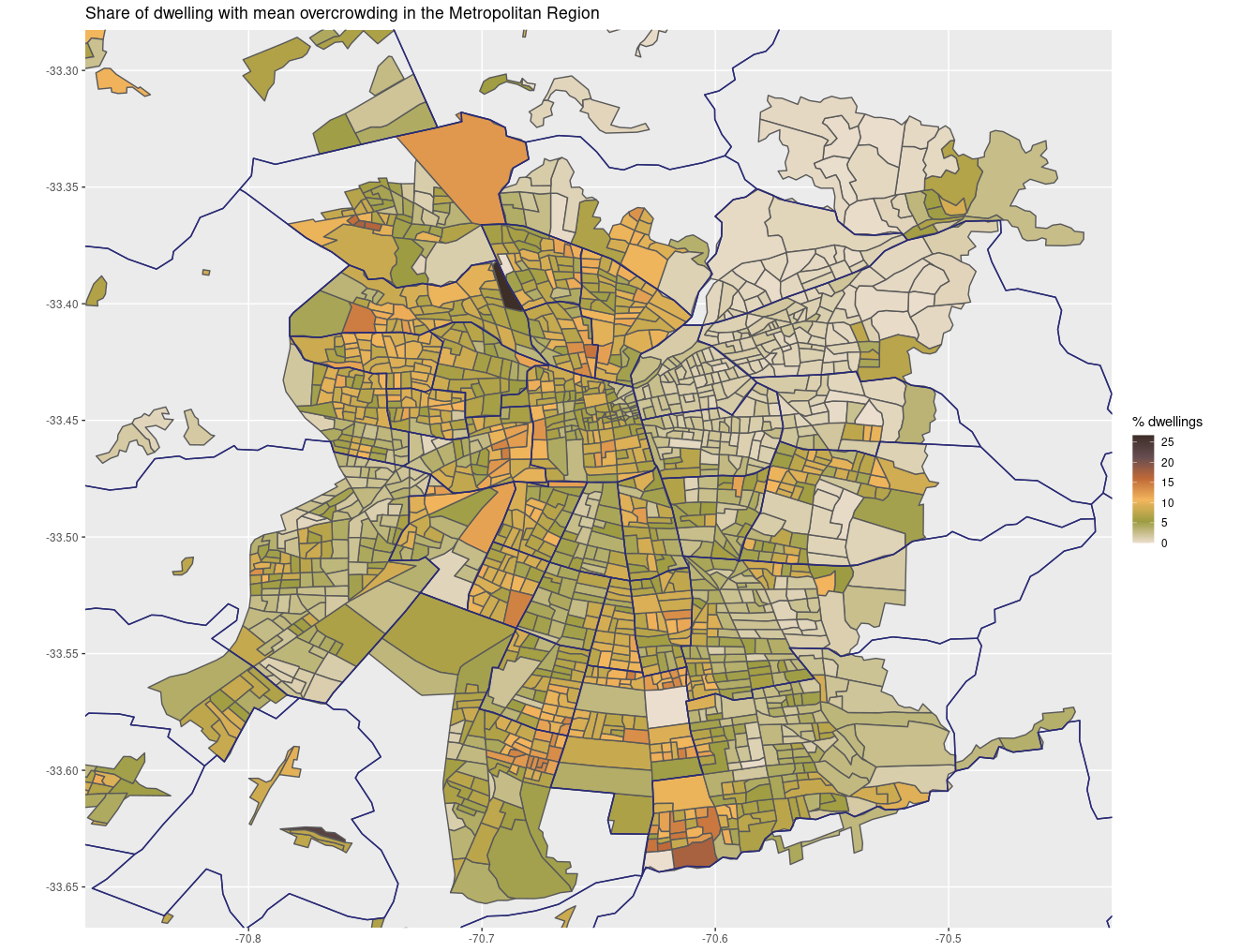

🔗Links to training and policy

Using open formats per se ease working as it reduces compatibility problems whenreading data, but datasets have to include proper documentation, not just comein proper formats. For the particular case of censo2017, it makes education andresearch resources more equitable, as it helps any institution that runs appliedstatistics courses or research to conduct census statistical analysis regardlessof the tools they use, and focus on a region or any group of interest, such asthe indigenous population, the elderly or the people living in apartments.

The census database I provide within the package can be read in Python, JavaC++, node.js and even right away from a command line, and it is important tomention that it's multiplatform. For the case of GUI-based applied statisticalanalysis, censo2017 makes it very easy to export subsets to Microsoft Excel orGoogle Sheets, without the disadvantages of the original census formatpreviously discussed, and even to Stata and SPSS thanks to the R packagesecosystem.

Those who, like me, write R packages can to do our contribution by creatingtools that could support the countries in the region to get back on track toachieving the Sustainable Development Goals defined by the United Nations, evenin spite of the recent rise of protectionism, political uncertainty and unclearattitude towards global trade regime seen in Latin America. Developing andenacting thoughtful policy is the only way to say 'checkmate' tounderdevelopment.

🔗rOpenSci community contribution

The help of rOpenSci and its softwarereview was pivotal.Dedicated reviewers, María Paula Caldas, Fransvan Dunné and MelinaVidoni, tested the package and suggested enhancements.Their reviews were very helpful, they gave extremely valuable advice and werereally supportive of my work and the development of the package.

The interested reader shall find a complete record of all the changes madeduring the reviewing process, where everything is commented in Spanish, andthere shall be newer rOpenSci packages in languages other than English. Since2011, rOpenSci has been creating technical infrastructure in the form of Rsoftware tools that lower barriers to working with scientific data. I can onlyremember the talk by my friend and colleague RivaQuiroga,where she highlights that initiatives such as this are not just software, buttools to make the community stronger.

I'd love to see different 'forks' of censo2017 in the contiguous countries Peruand Bolivia, and the rest of the region. Creating the first rOpenSci packagefully documented in Spanish is not just about inclusiveness, which is obviouslydesirable. This is also related to productivity, because in Latin Americamaterials that are documented in English are hard to understand and thereforethe tools are not adopted as one would want. And just like the infrastructurefor R4DS in Spanish motivated the creation of R4DS in Portuguese, I hope thatcenso2017 opens the door for interesting collaborations and similar packages indifferent languages.

I think I do my best to contribute to initiatives such as rOpenSci because hereI have found my place and discovered others who have a heartfelt wish to learnat many different things. My present contribution is makingthe right data, tools and best practices more discoverable while contributingto social infrastructure at the same time.